Making the Middle Count

You are hopefully confident your squad will score highly in each gameweek and given your transfer limitations, perhaps also in a few gameweeks to come. How can you be confident in this? What are the factors you should consider before selecting your squad? These are the ideas we need to quantify before we can move on to any kind of machine learning. In this post I will talk about the general squad structure I aim for and introduce a program I use to optimise this.

After playing FPL for a number of years, I have developed a squad structure which I am happy with and rarely diverge from. Usually I have:

1. Two starting goalkeepers outside the “Big Six”. In recent years I have found “Big Six” goalkeepers overpriced and having two mid-table goalkeepers to rotate with respect to favourable fixtures is usually the better option and allows you to spend money elsewhere.
2. Three premium defenders. These players are usually accompanied by a price tag of £5.5m+, but have proven well worth the investment in recent years. In todays football, we see fullbacks bombing forwards and the likes of Alonso, Robertson, Trippier and Mendy have all been excellent selections this year.
3. Two budget defenders. With the three premium options, there is no need to throw any more cash on the backline. Wan-Bissaka and Bennett always play for their respective teams and with their modest price tag of around £4.0m, they have been trustworthy substitutes for me this season.
4. Three premium options. The squad is not complete without your Hazards, Agueros, Salahs, and Kanes. This is where you expect to get the big points.
5. The rest. There are five picks left spanning the attack and midfield. Usually, I select these in the £5.5m-£7.5m range depending on how much I have spent on the above. I will refer to these as the middle men and today we are going to make them count.

Below is a picture of my squad going into gameweek 16. Hopefully the structure mentioned above is clear.

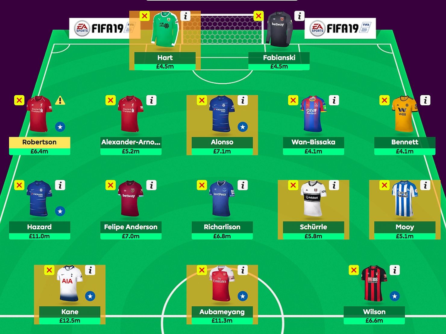
Unless they have particularly favourable fixtures, Wan-Bissaka and Bennett tend to sit on the bench. The key decisions to make is who out of the middle men joins them. For gameweek 16, it looks like it might be Mooy, as Huddersfield face Arsenal away.

For any FPL analysis, thinking about upcoming fixtures is crucial and the table below outlines how difficult I believe each team is to face home and away (higher score = harder).

Difficulty	MCI	LIV	CHE	TOT	ARS	MNU	WOL	EVE	WHU	BOU	LEI	WAT	BHA	BUR	CRY	NEW	FUL	SOU	HUD	CAR
Home	80.0	73.0	71.0	70.0	63.0	62.0	55.0	51.0	50.0	46.0	46.0	44.0	42.0	42.0	42.0	40.0	39.0	38.0	34.0	33.0
Away	104.0	94.9	92.3	91.0	81.9	80.6	71.5	66.3	65.0	59.8	59.8	57.2	54.6	54.6	54.6	52.0	50.7	49.4	44.2	42.9

The figures have simply been derived from looking at what betting companies think along with personal judgment. Analysing fixture difficulty is a topic in itself and will be covered in a later post. For the purpose of this post, the numbers above will suffice.

When picking your middle men, it is slways desirable to have the option to field four with decent fixtures over the next few gameweeks. The player with the hardest fixture each gameweek doesn’t matter too much, as he will sit on the bench. Hence, how strong your middle men are is a function of the four easiest fixtures over next few gameweeks. Lets apply this reasoning to my middle men.

The table below displays the difficulty of the next five fixtures played by my middle men. The fixture highlighted in red, is the toughest each gameweek and if no transfers are made over the period, the player with the red fixture will be put on the bench. The sum of the the non coloured cells represent how strong my middle men are, in this case it’s 1061.3. A lower value is better.

Table 1. The fixture difficulty of my middle men.

Player	GW16	GW17	GW18	GW19	GW20
Wilson	73.0	71.5	42.0	91.0	80.6.0
Richarlison	44.0	104.0	70.0	54.6	54.6
Schurle	80.6	50.0	52.0	55.0	34.0
Mooy	81.9	40.0	38.0	80.6	50.7
Felipe Anderson	42.0	50.7	44.0	49.4	54.6

The code

It would be useful to calculate the above score for all possible combinations of five middle men. This will be the the goal of this section.* It is of course not necessary to consider all midfielders and forwards in the £5.5m-£7.5m range, but perhaps a subset of players who are in good form and are likely to play well going forward. I have decided to look at players who have at least 48 total points or 5 in the FPL form rating. The table below displays which teams have players under this condition. In total, there are 30 players we wish to consider.

	ARS	BOU	BHA	BUR	CAR	CHE	CRY	EVE	FUL	HUD	LEI	LIV	MCI	MNU	NEW	SOU	TOT	WAT	WHU	WOL
Players	0	3	2	1	1	3	2	3	2	1	1	2	1	0	1	2	1	1	2	1

I have written a program in R with the above details and highlighted goal in mind. Lets break this program down and comment on some of the results.

#Adding number of interesting players
FPL[["Players"]] <- c(0,3,2,1,1,3,2,3,2,1,1,2,1,0,1,2,1,1,2,1)

#Removing teams with no interesting players
FPL <- FPL[!(FPL$Players==0),]
#Rearranging DF
FPL <- FPL[,c(1,40,2:39)]

#Making vector containing all the player teams
TeamsVector <-c()
for(i in 1:length(FPL$Team)){
  j <- cumsum(FPL$Players)[i]-FPL$Players[i]
  for(k in 1:FPL$Players[i]){
    TeamsVector[j+k] <- FPL$Team[i]
    }
}

#Making matrix containing all five player combinations
PlayerMatrix <- t(combn(TeamsVector,5))

GwStart = 16 #First gameweek we consider
GwEnd = 20 #Last gameweek we consider
n = GwEnd - GwStart + 1 #Number of games we are looking at

#Making DF only including gameweeks we consider
FPL2 <- FPL[c(1,(GwStart+2):(GwEnd+2))]

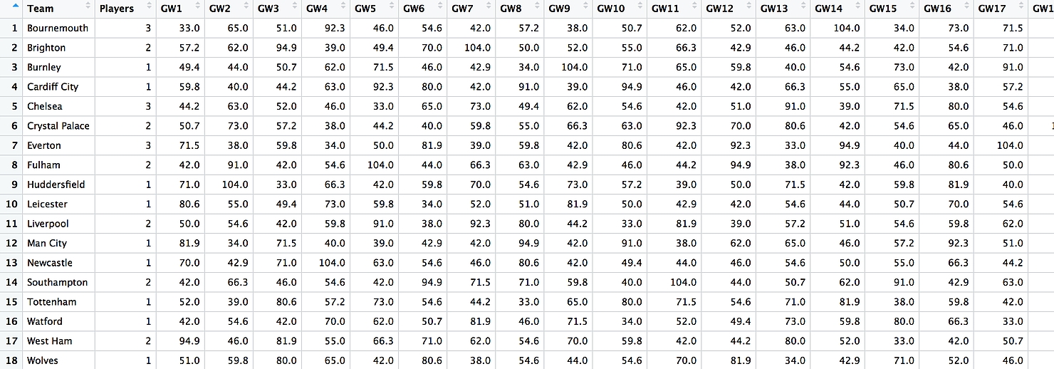
The output from the above code is “FPL”, a dataframe which only includes teams with players we wish to consider, how many interesting players there are in each team and the difficulty for these teams. See Figure 1 of the Appendix. “FPL2” later becomes the equivalent dataframe only including the gameweeks we wish to consider.

The vector “TeamsVector” contains all the players we wish to consider. So far, we don’t distinguish between players in the same team. So even though Wilson and King are interesting players, they both appear as “Bournemouth” in TeamsVector.

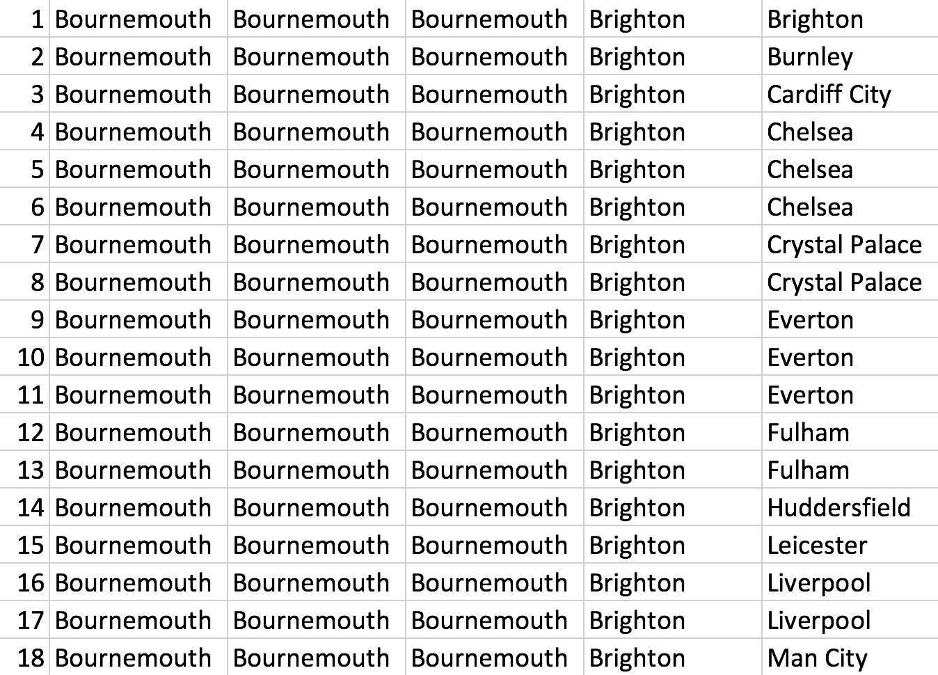
The rows in the matrix “PlayerMatrix” add up to all five player combinations taken from the set of our 30 interesting players. The matrix has ${30 \choose 5} = 142506$ rows and the first few are displayed in Figure 2 of the Appendix. Note that rows 5 and 6 are the same. This is because we are considering two players from Chelsea.

Below we introduce some functions which will be useful for our analysis. I will first present the code and then explain their structure.

SumMinusMax <- function(x){
  #Takes numeric vector and returns the cumulative value minus the largest value
  return(sum(x)-max(x))
}

MatrixMaker  <- function(L,DataFrame,n=5){
  #takes a list of teams and a date frame and produces a matrix with their game difficulties. n is the number of gameweeks we are looking at.
  v1 <- as.numeric(DataFrame[match(L[1],DataFrame$Team),c(2:(n+1))])
  v2 <- as.numeric(DataFrame[match(L[2],DataFrame$Team),c(2:(n+1))])
  mat <- matrix(c(v1,v2),nrow=length(v1))
  for(i in 3:length(L)){
    vi <- as.numeric(DataFrame[match(L[i],DataFrame$Team),c(2:(n+1))])
    mat <- cbind(mat,vi)
  }
  return(t(mat))
}

Score <- function(M) {
  #Takes a matrix and return the sum of the SumMinusMax values of the columns
  Ans <- 0
  for(i in 1:ncol(M)){
    Ans <- Ans + SumMinusMax(M[,i])
  }
  return(Ans)
}

“SumMinusMax” is very simple. It takes any numeric vector, finds its cumulative value and subtracts its largest value.

“MatrixMaker” produces a matrix similar to the one in Table 1 above. Given a list of five teams, it produces a matrix with the teams fixture difficulty over the next n games. The variable “DataFrame” needs to be in the form of FPL2.

“Score” takes a matrix as the one produced by MatrixMaker and returns the score of that set of middle men. Our goal is to apply MatrixMaker to all our rows in PlayerMatrix, followed by the Score function. The code below does this and stores the results in the vector “Scores”.

#Filling the vector Scores with the scores for the the set of players in the PlayerMatrix
Scores <- c()
for(i in 1:nrow(PlayerMatrix)){
  Scores[i] <- Score(MatrixMaker(PlayerMatrix[i,],FPL2))

}

#Add the scores to the PlayerMatrix and a couple of interesting stats
Ans <- cbind(PlayerMatrix, Scores, rank(Scores),rank(Scores)/length(Scores))

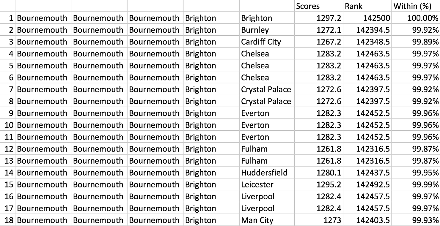
In Ans, we combine “Scores”, a couple of useful stats and PlayerMatrix. The result is seen in Figure 3 of the Appendix.

Results

The table below shows row 20939 of Ans which happens to be the combination of middle men I currently possess and we can hence conclude that my boys are within the top 26% of all combinations. Luckily the score of 1061.3 is consistent with what we had before.

Player 1	Player 2	Player 3	Player 4	Player 5	Scores	Rank	Within (%)
Bournemouth	Everton	Fulham	Huddersfield	West Ham	1061.3	36218	25.42%

Perhaps this suggests that my middle men are an area where we can improve my squad. If we were to change Wilson for Chicharito, we score 980.3 and fall within the top 0.3% instead. The strongest combination is shown in the table below.

Player 1	Player 2	Player 3	Player 4	Player 5	Scores	Rank	Within (%)
Fulham	Southampton	Watford	West Ham	West Ham	948.8	2.5	0.00%

A possible set of players which achieve this are Mitrovic, Armstrong, Pereyra, Felipe Anderson and Chicharito.

Improvements

Lets think about how we can improve the model!

Improvements to outputs in Ans:

• Ans could be made to distinguish between players in the same team. Rather than listing teams, players could be listed and perhaps also their total cost.

Improvements to model:

• Rather than using somewhat arbitrary values for fixture difficulty, clearly a model could be made to derive these. As mentioned, this will be covered in another post.
• The fixture difficulty could be player dependent as well as team dependent. In this case, line 7 and 8 in Figure 3 of the Appendix might get a different score if one of the Crystal Palace players is in better form than the other.
• The model could take into account what players already exist in the squad and hence only consider combinations of middle men which fall within the remaining budget and available places. This reduces computation time and provides a clearer view of the options available.

Appendix

Figure 1. Dataframe after deleting teams with no interesting players and some rearranging.

Figure 2. The first 18 rows of PlayerMatrix.

Figure 3. The first 18 rows of Ans