Dixon Coles Model

In 1995 Mark Dixon and Stuart Coles were fed up with football results being predicted by Poisson models. Because lets be honest, they probably can’t. So here it is, the new and improved Dixon Coles model suitably named after the two authors. If not only for amusing quotes such as “A recently introduced type of betting, fixed odds betting, is also growing in popularity. Bookmakers offer odds on the various outcomes of a match” which reveals how ancient the paper is, it is certainly worth a read. The paper suggests two improvements to the standard Poisson model which will be discussed here. As a refresher, please do head up to the header for a link to my post on Poisson models.

Low Scoring Games

The heart and soul of the Poisson model is that the number of goals scored by each team can be modeled by two independent, you guessed it, Poisson distributions. At the start of the paper, Dixon and Coles discuss the suitability of this independence assumption and argue that it is not suitable for low scoring games. There seems to be some evidence for this theory in practice. Below is a heat map, courtesy of David Sheehan author of an excellent blog, which displays the average difference between actual and Poisson model predicted scorelines for the 2005/06 season all the way up to the 2017/18 season. Green cells imply the model underestimated those scorelines, while red cells suggest overestimation - the color strength indicates the level of disagreement.

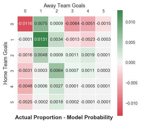
Indeed, there are issues around low scoring draws but there is little to say about 1-0 and 0-1. In the light of this, Dixon and Coles introduce the dependence factor, $\tau$, which takes the following form in the models probability distribution:

$$\begin{align*} P(X_{i,j}=x,Y_{i,j}=y) &= \tau_{\lambda, \mu}(x,y)\frac{e^{-\lambda} \lambda ^x }{x!}\frac{e^{-\mu} \mu^y }{y!} \\ \lambda &= \alpha_{i}\beta_{j}\gamma \\ \mu &= \alpha_{j}\beta_{i} \\ \tau_{\lambda, \mu}(x,y) &= \begin{cases} 1-\lambda\mu\rho& \quad \text{if }x=y=0 \\ 1+\lambda\rho& \quad \text{if }x=0,y=1 \\ 1+\mu\rho& \quad \text{if }x=1,y=0 \\ 1-\rho& \quad \text{if }x=y=1 \\ 1& \quad \text{otherwise.}\\ \end{cases} \end{align*}$$

Here $X$ and $Y$ are the home and away goals scored, $\alpha_{i}$ and $\beta_{i}$ are the home team attacking and defensive strength and equivalently for the away team $j$. $\gamma$ is the home team advantage factor and $\rho$ is the newly introduced dependance factor. Setting $\rho = 0$ corresponds to independence. In our work going forward, we will aim to estimate a non-zero value for $\rho$ which deals with the issues we have for low scoring games. In practice, $\tau$ multiplies our low scorline probabilities with a non unit value. The model remains Poisson for high scoring games. Given that $\rho$ is expected to be small, this is really a very minor correction.

Time Decay

Manchester City loosing 3-2 against Norwich yesterday is more interesting to us than City beating Stoke 7-0 two years ago with regards to estimating the current attack and defensive strength of City. This is not taken into account at the moment. In fancy words: The current model is static - the attack and defense parameters of each teams are regarded as constant throughout time. Lets fix that!

Lets start by ignoring the above statement. As it stands, we have $2n + 2$ parameters to estimate, where $n$ is the number of teams in our dataset, 20 for the Premier League. $n$ $\alpha$’s, $n$ $\beta$’s, $\gamma$ and $\rho$. When estimating parameters we often refer to the likelihood of our observations and try to maximize this through varying our parameters. In simple terms: A bunch of games have been played, what values do we give our parameters so that the outcome of the games played were actually very likely to happen in the first place? In even simpler terms: Sophie scored 5 goals in every single game she played last season. We want to model her scoring rate with a Poisson distribution. Sophies Poisson parameter is probably about 5, not 1. Likelihoods are a key concept in probability theory and in this post going forward. Read up about that here.

In our case, the likelihood function takes the following form:

$$\begin{align*} L(\alpha_i, \beta, i, \gamma, \rho, i=1,...,n) &= \prod_{k=1}^{N} P(X_{i(k),j(k)}=x_k,Y_{i(k),j(k)}=y_k) \\ &= \prod_{k=1}^{N} \tau_{\lambda_k, \mu_k}(x_k,y_k)\frac{e^{-\lambda_k} {\lambda_{k}}^{x_k} }{x_k!}\frac{e^{-\mu_k} {\mu_{k}}^{y_k} }{y_k!} \\ &\propto \prod_{k=1}^{N} \tau_{\lambda_k, \mu_k}(x_k,y_k)e^{-\lambda_k} {\lambda_{k}}^{x_k} e^{-\mu_k} {\mu_{k}}^{y_k} \end{align*}$$

In the likelihood function, $k$ runs through all N matches in our dataset and multiply these together given our parameters where $\lambda_k = \alpha_{i(k)}\beta_{j(k)} \gamma$ and $\mu_k = \alpha_{j(k)}\beta_{i(k)}$ are match dependent for home team $i$ and away team $j$. In the final step above we have simply got rid of the factorial factors as these just combine to one very very big number which becomes irrelevant when we’re trying to maximize the likelihood with respect to the parameters.

To maximize, we find the partial derivatives of $L$ with respect to the parameters (gradient if you will). This looks incredibly scary and a common trick in this case is to consider $\log_e(L)$ instead. This works since the $\log$ function is a monotonically increasing function (ie, it increases as its argument increases), hence the maximums of $L$ are the same as those for $\log_e(L)$. The gain here is that logs of products become sums, which are much easier to deal with. the log likelihood is:

$$\begin{align*} LL(\alpha_i, \beta, i, \gamma, \rho, i=1,...,n) &= \sum_{k=1}^{N} \log(\tau_{\lambda_k, \mu_k}(x_k,y_k))-\lambda_k+x_k\log(\lambda_k)-\mu_k+y_k\log(\mu_k) \end{align*}$$

Going back to the first paragraph, our goal was to impose some sort of time dependance where more recent games are given more weighting. A good idea which achieves this is to multiply each term in the log likelihood by a monotonically decreasing function of time (ie a function that decreases with time). Here, $t$ for game $k$ is the time in days since the game was played. $\phi(t) = -t$ is monotonically decreasing, but for things to look pretty, we want a function that is 1 at $t=0$ and strictly positive… lets throw $\phi(t) = e^{-\epsilon t}$ for some positive constant $\epsilon$ in there. The size of $\epsilon$ dictates how quickly the importance of older games deteriorates. This is illustrated below.

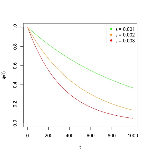
It is a little problematic finding an optimal value for $\epsilon$. Dixon and Coles choose $\epsilon$ to optimize outcome predictions (win, loss, draw) rather than actual scorelines, which simplifies things slightly. In their paper, they use half week units for t and arrive at a value of 0.0065 for $\epsilon$. For us, that translates to $\frac{0.0065}{3.5} = 0.0019$. In the interest of keeping this post within a 30 min read, we are going to take this value as gospel. Adding the time decaying weighting function, our log likelihood becomes:

$$\begin{align*} LL(\alpha_i, \beta, i, \gamma, \rho, i=1,...,n) &= \sum_{k=1}^{N} e^{-\epsilon t}[\log(\tau_{\lambda_k, \mu_k}(x_k,y_k))-\lambda_k+x_k\log(\lambda_k)-\mu_k+y_k\log(\mu_k)] \end{align*}$$

Below is some code which encapsulates the above. MatchLL finds the contribution to the total log likelihood from any one game. This is then used in LL which finds the total log likelihood of our dataset given some vector of parameters.

$$\begin{align*} \text{Parameters} &= \begin{bmatrix} \alpha_{1}, ..., \alpha_{n}, \beta_{1}, ..., \beta_{n}, \gamma, \rho \end{bmatrix} \end{align*}$$

The parameters are in alphabetical order which means that for the Premier League $\alpha_{1}$ corresponds to the attacking strength of Arsenal. Match_Data is a dataframe with all Premier League Fixtures since the start of the 17/18 season. As usual, this data is taken from football-data.co.uk.

tau <- Vectorize(function(x, y, lambda, mu, rho){
  #Defining the tau function
  if (x == 0 & y == 0){return(1 - (lambda*mu*rho))
  } else if (x == 0 & y == 1){return(1 + (lambda*rho))
  } else if (x == 1 & y == 0){return(1 + (mu*rho))
  } else if (x == 1 & y == 1){return(1 - rho)
  } else {return(1)}
})

phi <- function(t, epsilon = 0.0019){
  # Defining the weight function
  return(exp(-epsilon*t))
}

MatchLL <- function(x,y,ai, aj, bi, bj, gamma, rho, t){
  # A function which calculates the log likelihood of some game
  lambda <- ai*bj*gamma
  mu <- aj*bi
  return(phi(t)*sum(log(tau(x, y, lambda, mu, rho)) - lambda + x*log(lambda) - mu + y*log(mu)))
}


LL <- function(Match_Data, Parameters){
  # Function which calculates the LL for all the games
  LL <- 0

  Teams <- sort(unique(Match_Data$HomeTeam))

  # Fixing gamma and rho, as these are constant for all games
  gamma <- Parameters[2*length(Teams)+1]
  rho <- Parameters[2*length(Teams)+2]

  for(k in 1:nrow(Match_Data)){
    # Finding index for the home and away team
    IndexHome <- match(Match_Data$HomeTeam[k],Teams)
    IndexAway <- match(Match_Data$AwayTeam[k],Teams)

    # Finding relevant Parameters and other variables
    ai <- Parameters[IndexHome]
    aj <- Parameters[IndexAway]
    bi <- Parameters[IndexHome + length(Teams)]
    bj <- Parameters[IndexAway + length(Teams)]
    t <- Match_Data$t[k]
    x <- Match_Data$FTHG[k]
    y <- Match_Data$FTAG[k]

    #Adding the LL from game k to the total
    LL <- LL + MatchLL(x,y,ai, aj, bi, bj, gamma, rho, t)
  }

  return(LL)
}

Maximizing the Log Likelihood

Next we need to find the parameters which maximize the log likelihood. In an ideal world we would do this analytically by finding the gradient and setting this to zero, but due to the high dimensionality of the problem, we are restricted to numerical maximization. This will be done by gradient ascent, a cousin to the better known gradient descent. The two algorithms are really very similar as there is only a subtle sign change between the two. If you are unfamiliar with the concepts, read about gradient descent here and the difference between the two here. If you can’t be bothered, here is a crash course in gradient ascent: The gradient of any scalar function, say $F: \mathbb{R}^{n} \to \mathbb{R}$, always points towards a (local) maximum of $F$. Hence:

$$\begin{align*} F(x+a\nabla F(x)) > F(x), \end{align*}$$

for some sufficiently small and positive $a \in \mathbb{R}$.

In their paper, Dixon and Coles imposed the following condition on the attack parameters:

$$\begin{align*} n^{-1}\sum^{n}_{i=1} \alpha_{i} = 1. \end{align*}$$

Ie, the average attack parameter is 1. This condition is not strictly necessary, but ensures that we arrive at the same order of maximizing perimeters whenever we run the gradient ascent.

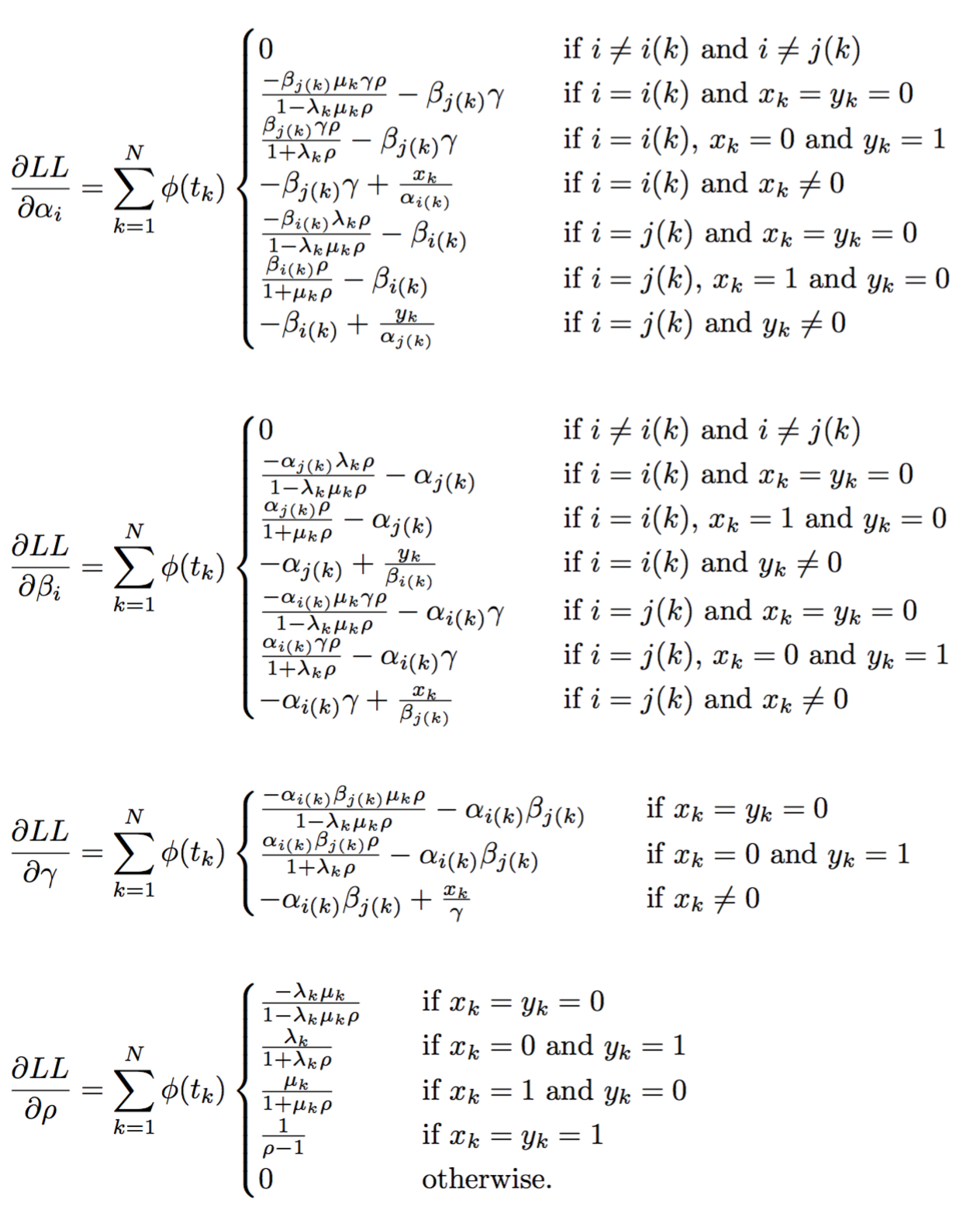
The first step in gradient ascent is to find the gradient of the log likelihood. To save you having to look at a sea of greek symbols, I have put these derivatives in the Appendix. Below is a rough sketch of the algorithm. The actual code can be found on my GitHub page.

#Optimise <- function(Match_Data)
# Creating Parameters, StartParameters and Gradient vectors of length 2n+2
# Setting all entries in Parameters to 1, apart from γ and ρ which are set to 1.3 and -0.05 respectively
#
# while(|Parameters - StartParameters| > Some small number)
#   Setting StartParameters = Parameters
#
#   Calculating the gradient of the log likelihood using Match_Data and Parameters using the partial
#   derivatives in the Appendix and setting equal to Gradient
#
#   Imposing the condition that the average attack parameter is 1. This is done by altering the gradient
#   in the following way:
#   Gradient = Gradient - Condition,
#   where Condition is a 2n+2 vector. Entries 1 to n are equal to the average of the first n entries in
#   Gradient. remaining entries are 0.
#
#   Setting PresentPoint = Parameters and
#   StepPoint = Parameters + Gradient
#
#   while(LL(Match_Data, StepPoint) > LL(Match_Data, PresentPoint))
#     Setting PresentPoint = StepPoint and
#     StepPoint = StepPoint + Gradient
#
#   Parameters = PresentPoint
#
# return(Parameters)

Before adding Gradient to StepPoint above, it is usual to reduce the size of Gradient so that the steps we take to locate the maximum aren’t too big, ie, we don’t want to miss it. This is done by multiplying Gradient by some constant smaller than 1, say $\theta$. $\theta$ is referred to as the step size and is allowed to change at every iteration. As we get closer to the maximum, usually we want $\theta$ to decrease.

It is somewhat arbitrary what we set $\theta$ as. For the purpose of what we’re doing, setting it equal to say $\frac{1}{100\times \text{length} (Gradient)}$ throughout the algorithm is fine. Although there are ways of setting $\theta$ to aid the speed of the algorithm. On my GitHub page, you will see that I have defined the function NMod which is used to decrease the size of Gradient as we approach the maximum.

As it stands, my algorithm takes about 10 seconds to optimize parameters to the closest 0.01. This time is of course dependent on the number of teams and and games in our dataset, but for comparison, there are functions in the alabama package such as auglag which I understand takes around 1 minute to run on a similarly sized dataset.

Results

As at 19 September 2019

Parameters

Team	α	β	Team	α	β
Arsenal	1.44	1.15	Man City	1.93	0.60
Aston Villa	0.56	0.96	Man United	1.26	0.97
Bournemouth	1.11	1.51	Newcastle	0.82	1.00
Brighton	0.68	1.26	Norwich	1.69	1.58
Burnley	0.87	1.24	Sheffield United	0.69	0.99
Cardiff	0.69	1.45	Southampton	0.87	1.32
Chelsea	1.28	0.98	Stoke	0.71	1.46
Crystal Palace	0.99	1.16	Swansea	0.57	1.23
Everton	0.98	1.09	Tottenham	1.38	0.85
Fulham	0.68	1.70	Watford	0.92	1.39
Huddersfield	0.48	1.50	West Brom	0.64	1.22
Leicester	1.04	1.08	West Ham	1.02	1,25
Liverpool	1.75	0.63	Wolves	0.94	1.12

$\gamma$ = 1.28 and $\rho$ = -0.06.

Conclusions

Firstly, lets have a couple of notes on the results:

• West Brom, Stoke, Swansea etc aren’t in the Premier League? Why do they appear in the results? That’s because they have been since the 17/18 season! Recall, our dataset goes two seasons back.
• Are Norwich really the third biggest attacking threat in the league? Probably not, but Norwich have only played 5 games in the Premier League over the last few years and putting three goals in against Man City (who according to the results have the strongest defense in the league) in the weekend will have boosted their attacking threat massively. I expect the attacking strength for Norwich to go down as the season progresses.

The Dixon Coles model is regarded as a pretty good one for football predictions. It is certainly good enough for our purpose which is to get a rough idea of which teams have favorable fixtures going forward and make FPL choices on the back of that. After speaking to friends who work in the industry, there are better models out there. These tend not to be published as companies use them to make serious money for themselves. For the time being, we will be using the Dixon Coles model going forward. My next to projects will most likely be to:

• Write a program which estimates the value for $\epsilon$ in the time decaying weight function.
• Use the model to find the expected number of goals scored by teams and the probability of holding clean sheets.

Stay tuned!

Appendix

The partial derivates of the log likelihood functions are below: