
“I will tell you how to become rich. Close the doors. Be fearful when others are greedy. Be greedy when others are fearful.” - Warren Buffett.
Ok, thats sounds easy enough and Warren Buffet arguably (not really) the most successful investor in the world, so we should probably listen to him. His quote above has been analyzed here, here and here and holds a lot more meaning than when people tell you to “Buy low and sell high”. Of course we all want to buy low, but how do we know when the market is low? Well, according to Mr Buffet, when people are fearful and vice verse for when the market is high. Fear and greed are emotions we can measure through reading The FT and talking to people. Hence, it can act as an investment strategy, “Buy low and sell high” can not. Even though a large proportion of the markets trading volume is driven by algorithmic trading, psychological and emotional factors still come into play. Conventional opinion on markets tend to rely on recent development. When market go up, investors become greedy and prices boil over, and one should be cautious lest they overpay for an asset that subsequently leads to anemic returns. When markets go down, and investors are fearful, it may present a good buying opportunity.
In this post I will take this idea and look to produce strategies which measures the optimism in market by looking at recent pricing and making investment decisions according. I will then post adds on dodgy websites saying “I hear this guy makes £5000 per month without leaving the house”
A Strategy
The key for the strategy is to measure the level of optimism in the market and invest and disinvest accordingly. Recent performance is the largest driver of market optimism. On the back of a few strong weeks, people tend to have optimistic views on the market and vice versa. The proposed strategy is a simple one and can be broken down into four points:
- We invest all our money into the market at time 0.
- Once the market goes down a
Sell_Numberof times, we sell all our holdings - Once the market goes up a
Buy_Numberof times, we invest all of our money in the market again - Each transaction costs an amount equal to
Cost_Per_Transaction. This is a set number, arguably it should be a percentage and could be easily changed to be just that.
To test the strategy we will run a bunch of pairs of Sell_Number and Buy_Number against the scenario when you invest at time 0 and keep your money invested. The market will be an index. In this post we will look at the FTSE 100, Nikkei 250 and Gold index. Here’s a bunch of code:
import pandas as pd
import numpy as np
# So that the whole np array is shown when printed
import sys
np.set_printoptions(threshold=sys.maxsize)

def Investment_Function(Index_List, Start_Money, Cost_Per_Transaction, Sell_Number, Buy_Number):
    """Function which takes an Index List, how much money you have to start with (float), the Cost per transaction (float), how many ups it takes for you to sell (int) and how many downs it takes for you to buy (int).
    Returns a matrix.
    First colum: Index
    Second column: Units held at each time,
    Third column: Value held at each time
    Fourth column: An explenation of what is happening"""

    # Making the units and value lists, filling with 0's. zerolistmaker is a function defined earlier in the module.
    Units = zerolistmaker(len(Index_List))
    Value = zerolistmaker(len(Index_List))
    Exp = zerolistmaker(len(Index_List))

    # Caluclating how many units we start with filling the first entries in the lists
    Start_Units = Start_Money/Index_List[-1]
    Units[-1] = Start_Units
    Value[-1] = Start_Money
    Exp[-1] = "Start"

    # "In" indicates if we are invested our not. "Count" will indicate how many ups/downs we have had in sucession
    In = True
    Count = 0

    # Working our way up the Index_List to work out when to buy and sell
    for i in range(-2,-len(Index_List)-1,-1):
        # We are In, Index goes up and we are below the selling point, so we dont sell
        if In and Index_List[i] > Index_List[i+1] and Count < (Sell_Number-1):
            Count += 1
            Units[i] = Units[i+1]
            Value[i] = Units[i]*Index_List[i]
            Exp[i] = "Up, but hold"
        # We are In, Index goes up and we hit the selling point, so we sell
        elif In and Index_List[i] > Index_List[i+1] and Count == (Sell_Number-1):
            Count = 0
            Units[i] = 0
            Value[i] = Units[i+1]*Index_List[i] - Cost_Per_Transaction
            # Returns 0 if we have run out of money
            if Value[i] < 0:
                Value[i] = 0
                Units[i] = 0
                return(np.column_stack((Index_List, Units, Value, Exp)))
            In = False
            Exp[i] = "Sell"
        # We are In, Index goes down, so we dont sell
        elif In and Index_List[i] < Index_List[i+1]:
            Count = 0
            Units[i] = Units[i+1]
            Value[i] = Units[i]*Index_List[i]
            Exp[i] = "Down, so hold"
        # We are not In, Index goes down and we we are bellow the buying point, so we don't buy
        elif not(In) and Index_List[i] < Index_List[i+1] and Count < (Buy_Number-1):
            Count += 1
            Value[i] = Value[i+1]
            Exp[i] = "Down, but don't buy"
        # We are not In, Index goes down and we hit the buying point, so we buy
        elif not(In) and Index_List[i] < Index_List[i+1] and Count == (Buy_Number-1):
            Count = 0
            Units[i] = (Value[i+1] - Cost_Per_Transaction)/Index_List[i]
            Value[i] = Value[i+1] - Cost_Per_Transaction
            # Returns 0 if we have run out of money
            if Value[i] < 0:
                Value[i] = 0
                Units[i] = 0
                return(np.column_stack((Index_List, Units, Value, Exp)))
            In = True
            Exp[i] = "Buy"
        # We are not In, Index goes up, so we don't buy
        elif not(In) and Index_List[i] > Index_List[i+1]:
            Count = 0
            Value[i] = Value[i+1]
            Exp[i] = "Up, so don't buy"
        # If the Index does not change, just copy what we had before
        elif Index_List[i] == Index_List[i+1]:
            Value[i] = Value[i+1]
            Units[i] = Units[i+1]
            Exp[i] = "Index unchanged"
        else:
            print("Something funny is happening at i =" + str(i))

    # Returning the matrix with Index Value, Units, Value and the explanation
    return(np.column_stack((Index_List, Units, Value, Exp)))
In addition to Sell_Number, Buy_Number and Cost_Per_Transaction as discussed above Investment_Function takes Index_List as a list of index values with the most recent value as its first entry. Start_Money is simply how much money we have to invest at time 0. The return is a matrix which illustrates how the strategy is progressing. I have managed to source the daily closing value of the FTSE 100 index between 20 October 1997 to 31 May 2019 from The London Stock Exchange. So lets look at an example where we have £10,000 to invest, the transaction cost is £1 and the Sell_Number and Buy_Number are both 2.
print(Investment_Function(FTSE100_Index, 10000, 1, 2, 2))
  ## ['4764.35' '1.94999951033' '9290.48016703' 'Buy']
  ## ['4863.79' '0.0' '9291.48016703' "Down, but don't buy"]
  ## ['4908.32' '0.0' '9291.48016703' "Up, so don't buy"]
  ## ['4897.43' '0.0' '9291.48016703' "Down, but don't buy"]
  ## ['4906.39' '0.0' '9291.48016703' "Up, so don't buy"]
  ## ['4842.33' '0.0' '9291.48016703' 'Sell']
  ## ['4801.92' '1.91901009783' '9214.93296898' 'Up, but hold']
  ## ['4755.39' '1.91901009783' '9125.64142913' 'Down, so hold']
  ## ['4840.72' '1.91901009783' '9289.39056077' 'Down, so hold']
  ## ['4970.2' '1.91901009783' '9537.86398824' 'Down, so hold']
  ## ['4991.47' '1.91901009783' '9578.68133302' 'Down, so hold']
  ## ['5148.76' '1.91901009783' '9880.52243131' 'Down, so hold']
  ## ['5225.91' '1.91901009783' '10028.5740604' 'Up, but hold']
  ## ['5211.02' '1.91901009783' '10000.0' 'Start']]
The table above gives the first 14 iterations of our strategy. Our initial £10,000 gives us approximately 1.92 units of the FTSE 100 index. After two successive ups in the index, we sell our holding at the 9th iteration and don’t invest again until 5 days later. The Sell_Number and Buy_Number are quite small for this strategy, so we will end up with quite a few transactions here. The transaction cost is illustrated nicely between the 13th and 14th iteration where our value has decreased by £1. Even though we have lost over £700 in two weeks here (ough), note that we are holding 0.03 units more compared to when we started. The strategy is therefore doing better than simply buying and holding which would results in a constant number of units held. This is because the transaction cost is trumped by the decreasing index between our Sell and Buy dates. Let’s look at how the strategy does over the full time horizon.
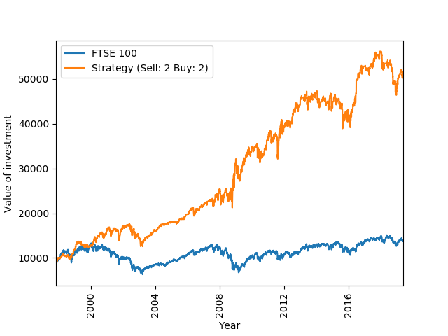
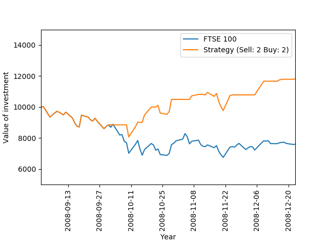
You can see how to produce these graphs on my GitHub page. The left image tells us that the strategy performs significantly better than the index over the full time horizon. Buying and holding takes our £10k to £14k whilst the strategy return £55k. Interestingly the strategy seems to to do particularly well during the 2008 financial crisis. This is a time where the index dropped significantly and we would not expect any strategy to do well. To illustrate this, the right image above plots the strategy had we invested in September 2008 until the end of the year. Since this is a shorter time period, we can now see buy and sell actions. The strategy is invested until the start of October. Subsequently, flat periods of the orange graph illustrate times when we are not invested. Over this period, the index dropped 24% whilst the strategy returned 20%. Interesting!
The next step is to work out which strategy like this is the most successful. To do so, firstly we need to consider which strategies are sensible to consider. Ie, it is not sensible to consider a strategy which sells after 25 ups, if the maximum number of successive ups is 10. The code below finds the maximum number of successive ups from an Index_List. There is an equivalent function for successive downs.
def Max_Ups(Index_List):
    """Function which takes a list of numbers and return the the maximum numbers of sucessive ups working from right to left"""
    Ans = 0
    Compar = 0

    # Working our way up the Index_List
    for i in range(-2,-len(Index_List)-1,-1):
        if Index_List[i] > Index_List[i+1]:
            Compar += 1
        else:
            Ans = max(Compar, Ans)
            Compar = 0

    Ans = max(Compar, Ans)
    return(Ans)
Below is a heat map illustrating how many times better each strategy does in comparison to buy and hold.
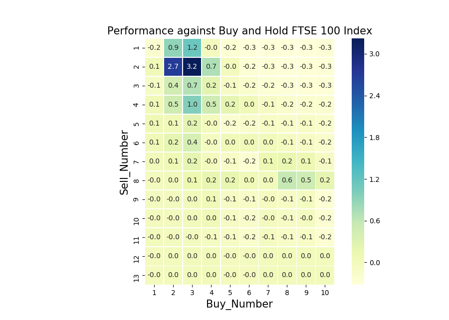
As usual, a recipe for the heat map is found on my GitHub page. Our Buy: 2, Sell: 2 strategy is the second most successful out of the bunch. Buy: 3, Sell: 2 is the best strategy and does 320% better than buy and hold. Ie, if the buy and hold strategy returned £100 after the time period, Buy: 3, Sell: 2 returns £420. Strategies which display 0 perform on par with buy and hold. Note that there are a bunch of these for high Sell_Numbers. For these strategies, you would rarely reach the high Sell_Number and you end up being invested for most of the time. This explains the on par performance. Relatively small Buy and Sell numbers seem to be the way to go in this example. Interestingly, there seems to be a cluster of stand out strategies around Buy: 8 and Sell: 8. Just out of interest, I have plotted Buy: 8 and Sell: 8 below.
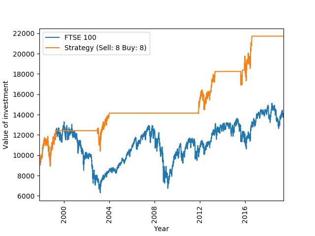
Due to the high Buy_Number, the strategy spends long periods out of the market, happens to spot 3 periods when the market does well and most importantly, misses the early 2000 and 2008 crashes. In addition, rather than just holding cash during the long periods where we are not invested, the strategy could invest straight into some form of fixed income, generating small but steady returns.
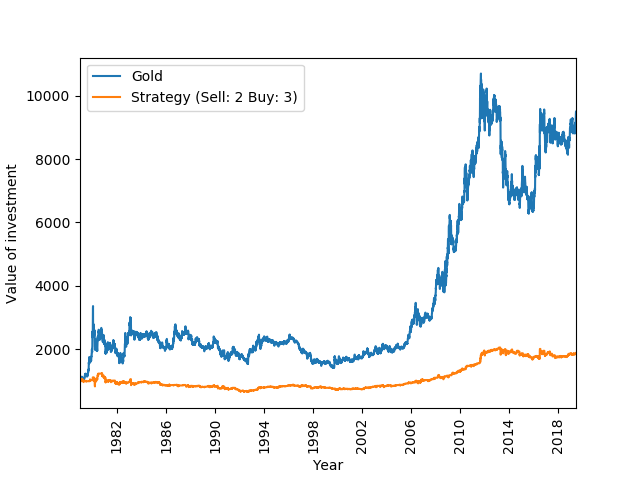
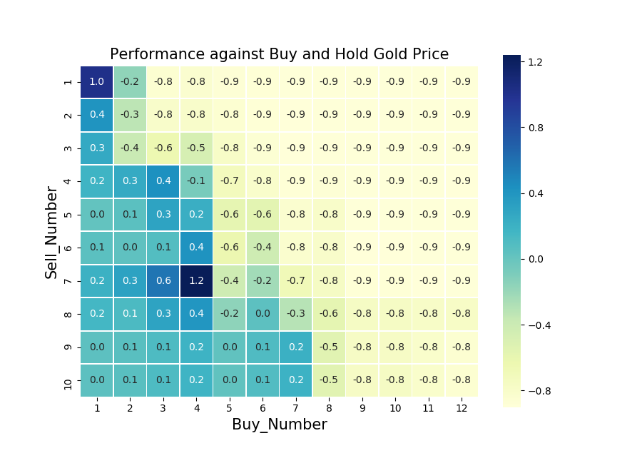
Now lets look at some other indices. Somewhat at random, I have chosen the Japanese Nikkei 225 stock index and the gold price index. Japanese stocks because they are one of the least correlated to UK stocks and gold, because, why not. I have found Nikkei 225 between 16 May 1949 to 14 June 2019 here and the gold price between 29 December 1978 to 7 June 2019 from here. Below I have plotted the Buy: 3, Sell: 2 strategy for both indices and their heat maps over the the full time horizon. For Nikkei 225 I have scaled the original investment down to £100 and £1000 for the gold price.
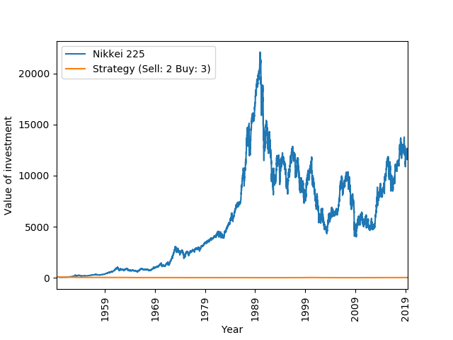
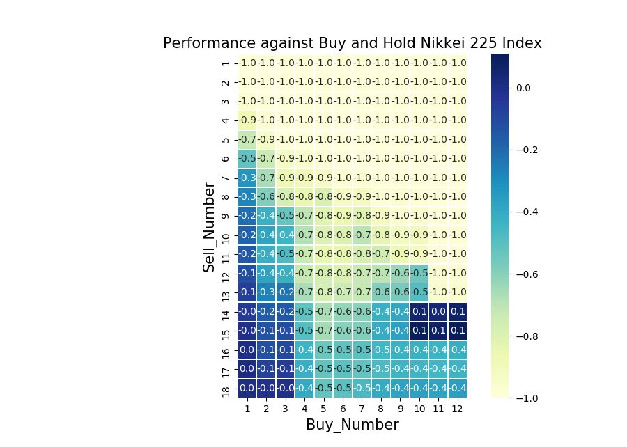
Whops, that doesn’t look too good… In the 40 years from 1950, the Nikkei 225 index appears to have increased almost exponentially. The annualized increase is in fact 15% over this period and there are only a hand full of years with negative returns. As a result, any strategy which does not stay invested in the index throughout this period is a bad one. This is painfully obvious looking at the heat map, showing that any strategy with a Buy_Number above 3 and Sell_Number below 14 does significantly worse than the index. It may not be obvious from the plot, but it is in fact the 1950s which yield the greatest returns. The annualized return was 23% over the decade and the index rose by almost 150% in 1952. As a result, all the strategies are doomed from the outset.
Albeit less prominent, there are similar periods of inflation in the gold price. However, there seems to be an area of positive return around Sell: 7, Buy: 4.
To look past these extreme conditions, below I have plotted the Sell: 2, Buy: 3 strategy (which was so successful for FTSE) against the Nikkei 225 index from the start of 1993 where the index follows trends normal by todays standards. To the left of this is the associated heat map.
As for the FTSE 100 Index the Sell: 2, Buy: 3 strategy does well and we see an area of positive returns in the top left corner of the heat map.
Another One
As discussed, we are trying to invest against public opinion. The fact that the first strategy makes decisions on the back of development over the last few days is fair criticism as public opinion may not have had time to form. Here is another strategy which hopefully solves that problem:
- We invest all our money into the market at time 0 and set
Lookbackequal to a certain number of days. - Once the market has returned a percentage equal or greater than
Sell_Percentageduring the course of aLookbackperiod, we sell. - Equivalent for
Buy_Percentage. - As before, we also have
Cost_Per_Transaction.
The code for this strategy is very similar for the one before and if you have understood the large block of code above, you could probably recreate it yourself. But for completeness, I have included it below.
def Investment_Function2(Index_List, Start_Money, Cost_Per_Transaction, Sell_Percentage, Buy_Percentage, Lookback):
    """Function which takes an Index_List, the money we start with, the transaction cost and our strategy.
    Sell_Percentage is float >0, Buy_Percentage is float <0.
    Returns a matrix with 5 columns
    Column 1: The index
    Column 2: Number of units held
    Column 3: Value of investment
    Column 4: What the comparsion is
    Column 5: An explanation of what is happening"""

    # Making the units and value lists, filling with 0's.
    Units = zerolistmaker(len(Index_List))
    Value = zerolistmaker(len(Index_List))
    Exp = zerolistmaker(len(Index_List))
    Comparison = zerolistmaker(len(Index_List))

    # Caluclating how many units we start with filling the first entries in the lists
    Start_Units = Start_Money/Index_List[-1]
    Units[-1] = Start_Units
    Value[-1] = Start_Money
    Exp[-1] = "Start"
    Comparison[-1] = 1.0

    # "In" indicates if we are invested our not.
    In = True

    # Working our way up the Index_List to work out when to buy and sell
    for i in range(-2,-len(Index_List)-1,-1):
        # We haven't gone far enough to start looking back
        if i>=-Lookback:
            Units[i] = Start_Units
            Value[i] = Start_Units*Index_List[i]
            Exp[i] = "Not gone far enough"
            Comparison[i] = 1.0
        # We can start building our comparison list
        else:
            Comparison[i] = Index_List[i]/Index_List[i+Lookback]
            # We are In and Index has done well enough over the Lookback, so we sell
            if In and Comparison[i] >= (Sell_Percentage+1):
                In = False
                Units[i] = 0
                Value[i] = Index_List[i]*Units[i+1] - Cost_Per_Transaction
                # Returns 0 if we have run out of money
                if Value[i] < 0:
                    Value[i] = 0
                    Units[i] = 0
                    return(np.column_stack((Index_List, Units, Value, Comparison,Exp)))
                    Exp[i] = "Run out of money"
                Exp[i] = "Index has done well, sell"
            # We are In and Index has not done well enough over the Lookback, so we do nothing
            elif In and Comparison[i] < (Sell_Percentage+1):
                Units[i] = Units[i+1]
                Value[i] = Units[i]*Index_List[i]
                Exp[i] = "Index has not done well enough to sell"
            # We are not In and Index has done poorly enough over the Lookback, so we buy
            elif not(In) and Comparison[i] <= (Buy_Percentage+1):
                In = True
                Units[i] = (Value[i+1]-Cost_Per_Transaction)/Index_List[i]
                Value[i] = Value[i+1] - Cost_Per_Transaction
                # Returns 0 if we have run out of money
                if Value[i] < 0:
                    Value[i] = 0
                    Units[i] = 0
                    return(np.column_stack((Index_List, Units, Value, Comparison,Exp)))
                    Exp[i] = "Run out of money"
                Exp[i] = "Index has done badly enough, se we buy"
            # We are not In and Index has not done poorly enough over the Lookback, so we do nothing
            elif not(In) and Comparison[i] > (Buy_Percentage+1):
                Units[i] = 0
                Value[i] = Value[i+1]
                Exp[i] = "Index has not done badly enough to buy"
            else:
                print("Something strange has happened")

    # Returning the matrix
    return(np.column_stack((Index_List, Units, Value, Comparison,Exp)))
A sensible number for Lookback may be around 30, which is what I will be using in this post. As before, to work out which strategies that are sensible to consider, we need to find the extreme values for Sell_Percentage and Buy_Percentage. A function which does this for Sell_Percentage is below.
def Max_Sell_Percentage_Func(Index_List, Lookback):
    """Function which takes an Index_List, Lookback and returns the maximum Sell_Percentage we could consider"""
    Comparison = zerolistmaker(len(Index_List))

    for i in range(-1,-len(Index_List)-1,-1):
        if i>=-Lookback:
            Comparison[i] = 1.0
        else:
            Comparison[i] = Index_List[i]/Index_List[i+Lookback]

    return(max(Comparison)-1)
Lets think of a sensible strategy. I don’t know…lets say that we went to sell or buy if the market has gone up or down by 4% over 30 days respectively. Lets plot this strategy with the associated heat map for the FTSE 100 and Nikkei 250 (post 1993) index.
Again, there is a cluster of blue tiles in the top left corner of the heat maps. Even though the particular Sell: 0.04, Buy: -0.04 strategy does not do well for Nikkei 250, there are strategies with larger Sell and Buy values that do. This is somewhat expected, since the Nikkei 250 Index is more volatile. On a side note, I am not sure why the column with Buy_Percentage equal to 0.00 is on the right hand side of the heat maps. The function used to make the heat maps is Make_Heatmap2() on my GitHub page, please feel free to have a look.
Conclusions
Investment managers are always careful to point out that past performance is not indicative of future results. I think we should point out the same cliché for the strategies we have tested. In both of our examples, we tested many variations displayed in the heat map. When these are all tested, some are going to look good, but this may be completely coincidental. To prove that it is not, any model that looks good (say Buy: 3, Sell: 2 for FTSE) would have to be tested further. I can think of two ways in which this can be done:
- Buy: 3, Sell: 2 does 320% better than the FTSE 100 Index over the full period. Fantastic! 1-0 to Buy: 3, Sell: 2. It would be even better if it also beats the Index every year (or at least in a vast majority of years) in the given time period. I don’t know if it does. It could be easily tested and would be a significant result if it turned out to be true. Every year in which Buy: 3, Sell: 2 wins gives another point to the strategy.
- The strategies could be tested against some Brownian motion with a general upwards trend. Brownian models are typically used to model stock prices. In using such a model we are not limited to historic data.
Another interesting point is that if the market is monotonically increasing, we can throw the strategies out of the window. In such a scenario, we are better off being invested all the time. This was painfully obvious in our first tests with the Nikkei 250 Index and Gold price. On the contrary, the strategies rely on bad times and actually flourish in these instances. This was investigated further in our analysis of the 2008 financial crisis and has a somewhat reassuring effect. The strategies can be relied on in gloomy times.
Have we found something here? I don’t know? Maybe?… Probably not? As it stands I wouldn’t be completely happy putting all of my money into one of these strategies. They definitely need more testing! But if nothing else, it is an interesting idea and I have enjoyed working around it. Thank you Mr Buffett.
Leave a comment